rm(list = ls())       ## create a clean environment

# create a dataframe called 'data'. The dataframe has 10 observations of 3 variables

data <- data.frame(
id = 1:10,
age = c(25, 31, 29, NA, 45, 38, NA, 52, 47, 33),
gender = c("M", "F", "F", "M", "F", NA, "M", "F", NA, "M")
)16 Data Pre_Processing - Practical
In the pre-class reading for this week, we covered three topics:
understand the importance of defining objectives for analysis
understand how to deal with missing data in R
understand how to identify, and deal with, outliers in datasets
In this practical, we’ll focus on the second and third of these.
16.1 Dealing with Missing Data
Failing to deal with missing data can basically invalidate our entire analysis.
16.1.1 Initial Phase
At this stage, we’re looking to see how much data is missing in our dataset, and where these gaps exist.
Usefully, in R, we can identify missing data using the is.na() function, which returns a logical vector of the same dimensions as your input data with TRUE values for missing data (represented as NA) and FALSE values for non-missing data.
Important
Note that R will usually enter ‘NA’ into the field of any missing data in an imported dataset. It’s important to check that this has happened when we first import the dataset (e.g., using the ‘head’ command or opening the dataset in a tab).
Here’s an example of identifying missing data in a dataset:
16.1.2 Identifying Missing Data
Technique 1 - using the is.na function
missing_data <- is.na(data)  # create a logical vector with TRUE or FALSE for each observation
print(missing_data) # show results in the console
id age gender
[1,] FALSE FALSE FALSE
[2,] FALSE FALSE FALSE
[3,] FALSE FALSE FALSE
[4,] FALSE TRUE FALSE
[5,] FALSE FALSE FALSE
[6,] FALSE FALSE TRUE
[7,] FALSE TRUE FALSE
[8,] FALSE FALSE FALSE
[9,] FALSE FALSE TRUE
[10,] FALSE FALSE FALSETechnique 2 - using the complete.cases function
complete.cases(data) [1] TRUE TRUE TRUE FALSE TRUE FALSE FALSE TRUE FALSE TRUE# shows whether each case is completed or not - printed to the console automaticallyTechnique 3 - also using the complete.cases function
data[!complete.cases(data),] id age gender
4 4 NA M
6 6 38 <NA>
7 7 NA M
9 9 47 <NA># This command shows the rows that have an NA in them. Note that we use the ! command in R to ask it find things that do NOT match our criteria, so in this case it has identified rows that are NOT complete cases.In the above example, the first option (using missing_data) created a logical matrix called ‘missing_data’ which has the same dimensions as data, with TRUE values for missing data (i.e. is missing) and FALSE values for non-missing data (i.e. is not missing).
From this new matrix, we can calculate the total number of missing values in the dataset:
total_missing_values <- sum(missing_data) # the sum command is used to calculate a total and put it into a new object
print(total_missing_values)
[1] 4We can calculate the number of missing values in each variable (column):
missing_values_per_variable <- colSums(missing_data)
print(missing_values_per_variable)
id age gender
0 2 2 We can also calculate the proportion of missing values in each variable. If a large proportion of values are missing from a particular variable, this may raise questions about its retention.
proportion_missing_values <- colMeans(missing_data)
print(proportion_missing_values)
id age gender
0.0 0.2 0.2 In this case, we can see that 20% of our cases (rows) have missing data in the ‘age’ variable, and 20% have missing data in the ‘gender’ variable.
These steps help you identify missing data in your dataset and to understand the extent of ‘missingness’ in your data. Depending on the amount and pattern of missing data, you can decide on the most appropriate way to handle the missing data.
16.1.3 Handle any missing values
If we’ve identified that we have missing data in our dataset, we now need to decide on the appropriate strategy to address missing data.
There are two main approaches to doing so:
One, called ‘imputation’, means that we create values and insert them in the missing spaces. We impute a value to replace the missing value.
The other approach is to remove records/observations where a missing value is present. In other words, if there’s a missing value, we ignore that observation (or delete it).
For the remainder of this module, we will assume that the best approach is ‘listwise deletion’. This means that we delete any observations (rows) where there is a missing value in any of the cells. The problem with this approach is that, in smaller datasets, it may mean we get rid of lots of observations, thus reducing our dataset to a dangerously small level.
The simplest way to carry out listwise deletion is with the na.omit command, as shown in the following code. You’ll see that it simply removes all the rows where there were missing values in **any* of the elements.
data01 <- na.omit(data)  # creates new datafame called data01 with only complete observations
print(data01)  # the resulting dataset is printed to the console.
id age gender
1 1 25 M
2 2 31 F
3 3 29 F
5 5 45 F
8 8 52 F
10 10 33 M
Note
In the previous example, I created a new dataframe called ‘data01’ which had the missing observations removed. This is better than simply overwriting the existing dataframe (‘data’) as I might wish to return to that original dataframe later in the analysis.
16.1.4 Conclusion
In this section, we’ve discussed two main things: how to identify if there is missing data present in our dataset, and how to remove any rows that contain missing data.
Remember: at this point, we’ve taken a ‘brute force’ approach to missing data, and removed any observations that have missing data within any of their elements. There are more sophisticated ways of dealing with this issue which we’ll cover in B1705.
16.2 Practice - Idenfifying Missing Data and Treatment
First, download the following dataset:
rm(list = ls())       ## create a clean environment
url <- "https://www.dropbox.com/scl/fi/90ipwg07sexckkpzy59h3/swim_data.csv?rlkey=gprb7p930dfs66w9xofcyxxz0&dl=1"
swimming_data <- read.csv(url)
rm(url)
Task One: Evaluate if missing data is a problem in this dataset.
Task Two: If missing data is a problem, create a new dataset called [swimming_data_nomissing] that contains only complete rows.
16.3 Outlier Detection
‘Outliers’ are data points that significantly differ from the rest of the data.
Detecting outliers is essential because they can have a strong influence on the results of data analysis and lead to misleading conclusions. However, it may not always be clear whether a value is a mistake, or if it represents a genuine observation.
There are two types of approach to inspecting for outliers - visual and statistical - that we can use to detect outliers in a dataset.
16.3.1 Visual methods
By plotting variables in the data, we can easily detect the presence of outliers. The most common methods used for this are box plots, scatter plots, and histograms.
We’ll start with a dataset:
# create a clean environment
rm(list = ls())

# set url for dataset
url <- "https://www.dropbox.com/scl/fi/jb9b9uhx728e4h6g46r1n/t10_data_b1700_02.csv?rlkey=3sjwjwd6y59uj5lq588eufvpm&dl=1"

# create a dataframe based on the file at the URL location
df <- read.csv(url)

# remove the url variable - we don't need it again
rm(url)
Box plots
Box plots give us a visual indication of a variable’s characteristics (25th percentile, 50th percentile, 75th percentile, minimum, maximum and maximum values). They also show any observations that lie ‘outside’ of that range.
# create boxplot for the variable Pl, part of the df dataset

boxplot(df$Pl, main = "Box Plot - Outlier Detection")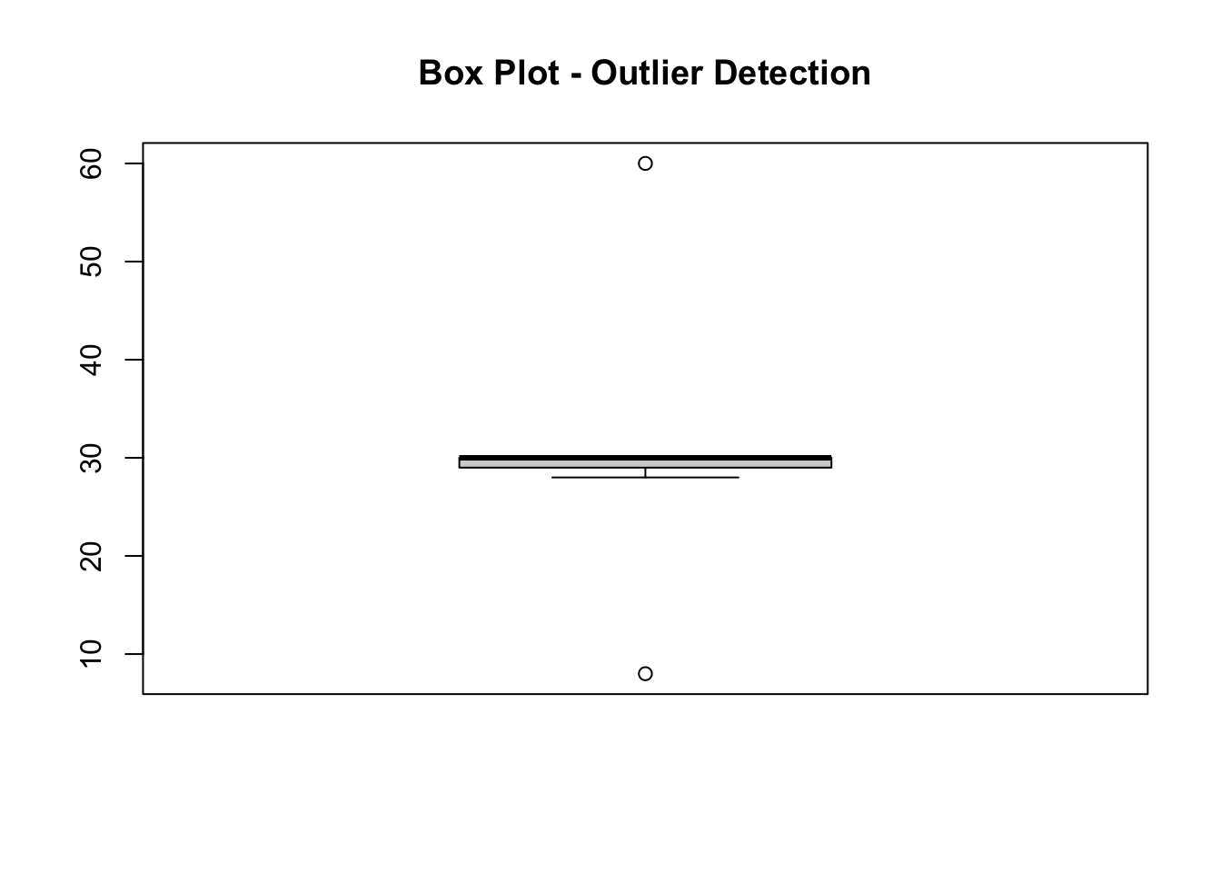
The resulting figure shows that there are two outliers within the variable ‘Pl’. One seems a lot greater than the rest of the observations, and one seems a lot less.
Scatter plots
In general a scatter plot is useful if you expect a general trend between two variables.
For example, in our dataset for the EPL, we’d expect a team’s position in the league and its total number of lost games to be negatively associated (higher position = fewer losses). If we find this isn’t the case for certain teams, it suggests an outlier in the data.
# create scatter plot and add labels for the x and y axes

plot(df$Pos, df$L, main = "Number of lost games by league position",
xlab = "League position", ylab = "Number of losses",
pch = 19, frame = FALSE)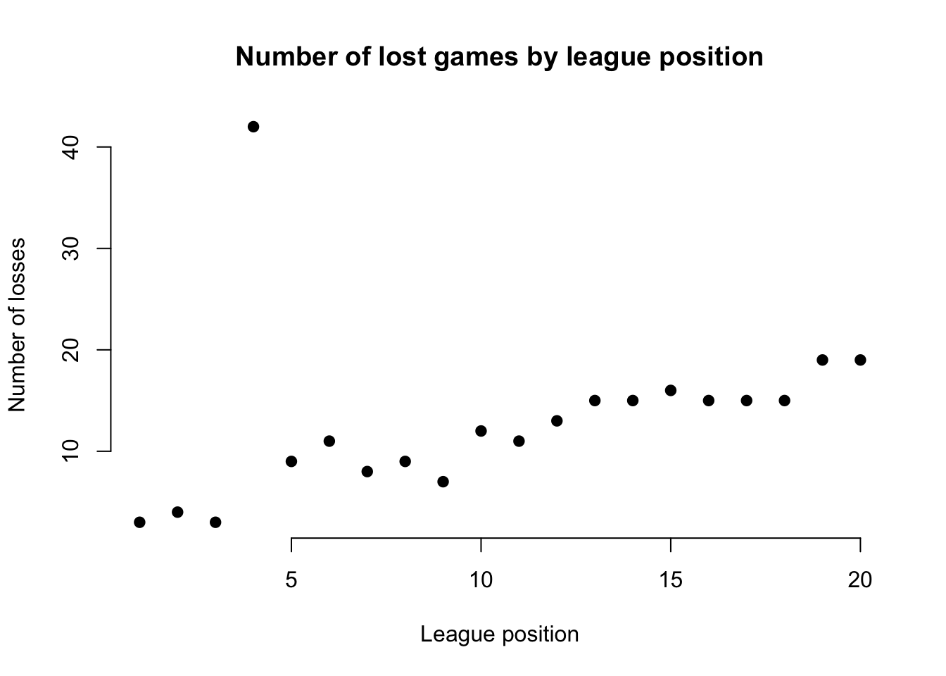
The resulting figure suggests an outlier in the data for the team at league position 4, whose number of lost games is far too high to be ‘reasonable’. It doesn’t mean it’s definitely an outlier, but it may suggest further inspection.
Histograms
The previous techniques work if we’re dealing with scale/ratio types of data. However, we also want to visually explore outliers in categorical or ordinal data.
Therefore, if we can make a reasonable assumption about the frequency of values in a variable, we can use a histogram to explore outliers in that variable.
For example, in the current dataset, we would assume that every team will have drawn a roughly similar number games. By creating a histogram, we can identify potential outliers.
# create histogram

hist(df$D, col = "steelblue")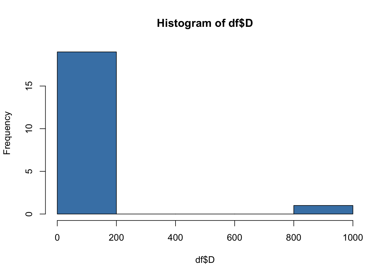
Clearly, there is a outlier in the ‘D’ variable! The x-axis shows that frequency of draws for most of our observations is in the range 0-200, while the frequency of draws for at least one of our observations is in the range 800-1000. We know that this cannot be correct!
Using the ‘summary’ command
We’ve covered three visual approaches to outlier detection that involved plotting graphs.
We can also visually inspect the descriptive statistics of our variables by running the summary command.
This gives us another way to quickly identify potential outliers, as can be seen for the ‘D’ variable in the following example, which has a maximum of 999, or the ‘Pl’ variable which indicates the number of games played, and you know that teams don’t play 60 games in a season.
summary(df) # run summary command on [df] dataframe Pos Team Pl W
Min. : 1.00 Length:26 Min. : 8.00 Min. : 6.00
1st Qu.: 5.75 Class :character 1st Qu.:29.00 1st Qu.: 7.75
Median :10.50 Mode :character Median :30.00 Median :10.00
Mean :10.50 Mean :30.05 Mean :11.30
3rd Qu.:15.25 3rd Qu.:30.00 3rd Qu.:14.25
Max. :20.00 Max. :60.00 Max. :23.00
NA's :6 NA's :6 NA's :6
D L F A
Min. : 4.0 Min. : 3.00 Min. :23.00 Min. :21.00
1st Qu.: 5.0 1st Qu.: 8.75 1st Qu.:28.25 1st Qu.:35.50
Median : 6.5 Median :12.50 Median :40.50 Median :40.00
Mean : 56.3 Mean :13.05 Mean :42.06 Mean :39.83
3rd Qu.: 9.0 3rd Qu.:15.00 3rd Qu.:49.50 3rd Qu.:42.75
Max. :999.0 Max. :42.00 Max. :75.00 Max. :54.00
NA's :6 NA's :6 NA's :8 NA's :8
GD Pts
Min. :-30.00 Min. :23.00
1st Qu.:-15.75 1st Qu.:29.75
Median : -1.50 Median :39.00
Mean : 0.00 Mean :40.90
3rd Qu.: 13.50 3rd Qu.:48.50
Max. : 48.00 Max. :73.00
NA's :6 NA's :6 16.3.2 Statistical methods
The previous methods depend on visual inspection.
A more robust approach to outlier detection is to use statistical methods. We’ll cover this in greater detail in B1705, but basically we are attempting to evaluate whether a given value is within an acceptable range. If it is not, we are making a determination that this value is probably an outlier.
There are two techniques we commonly use for this: z-scores, and the IQR.
z-score
Z-scores represent how many standard deviations a data point is from the mean.
A common practice is to treat data points with z-scores above a certain absolute threshold (e.g., 2 or 3) as outliers.
library(zoo) # load the zoo package
Attaching package: 'zoo'The following objects are masked from 'package:base':
as.Date, as.Date.numeric # first we create some data - a set of values that all seem quite 'reasonable'.
data <- c(50, 51, 52, 55, 56, 57, 80, 81, 82)
# then, we calculate the z-scores for each value
z_scores <- scale(data) # we scale the data
threshold = 2 # we set an acceptable threshold for variation
outliers_z <- data[abs(z_scores) > threshold] # we identify values that sit outside that threshold
print(outliers_z) # there are no outliers in the datanumeric(0)# Now, we introduce an outlier - 182 - to the vector [data]
data <- c(50, 51, 52, 55, 56, 57, 80, 81, 182)
z_scores <- scale(data)
threshold = 2
outliers_z <- data[abs(z_scores) > threshold]
print(outliers_z) # note that the outlier has been identified successfully[1] 182Interquartile Range (IQR)
The interquartile range tells us the spread of the middle half of our data distribution.
Quartiles segment any vector that can be ordered from low to high into four equal parts. The interquartile range (IQR) contains the second and third quartiles, or the middle half of your data set.
In this method, we define outliers as values below (Q1 - 1.5 x IQR) or above (Q3 + 1.5 x IQR).
# Calculate IQR of our vector

Q1 <- quantile(data, 0.25)
Q3 <- quantile(data, 0.75)
IQR <- Q3 - Q1

# Define threshold (e.g., 1.5 times IQR)
lower_bound <- Q1 - 1.5 * IQR
upper_bound <- Q3 + 1.5 * IQR

# Identify outliers
outliers <- data[data < lower_bound | data > upper_bound]

# Print outliers
print(outliers)  # the outlier of 182 has been successfully identified
[1] 182It’s important to note that these statistical methods rely on likelihood of the value being outside the ‘normal’ range. This means that ‘real’ values might accidentally be flagged as outliers…
16.3.3 Outlier Treatment
We need to tackle any outliers in our dataset.
Remove outliers
The easiest approach, as was the case with missing data, is to simply remove them.
Previously, we learned some approaches to visually identifying outliers. If we’ve done this, we can use the following process to ‘clean’ our data, because we know what the outlier value is.
data <- c(50, 51, 52, 55, 56, 57, 80, 81, 182)

# here I've used the ! command to say [data_clean] is [data] that is NOT 182
data_clean <- data[data != 182]
If we’ve visually identified an outlier and know its index (position), for example through a scatter plot, we can remove it using its index:
data <- c(50, 51, 52, 55, 56, 57, 80, 81, 182)
data_clean <- data[-9] # this creates a new dataframe without the 9th element
print(data_clean)
[1] 50 51 52 55 56 57 80 81If using z-scores, we can use the following process, which assumes a threshold of 2 (we can adjust this based on our needs). Now, we can remove data points with z-scores greater than 2 in absolute value.
Notice that this is more efficient, because we don’t need to tell R what the value/s of the outliers are.
data <- c(50, 51, 52, 55, 56, 57, 80, 81, 182) # Example data with the 182 outlier
z_scores <- scale(data) # calculate z-scores
threshold = 2  # set threshold
data_cleaned <- data[abs(z_scores) <= threshold] # create a 'clean' set of data
print(data_cleaned) # the outlier has been removed
[1] 50 51 52 55 56 57 80 81Finally, we may want to remove all observations in the dataframe that contain an outlier. This is helpful if we wish to retain the integrity of the dataframe rather than dividing it up into seperate vectors.
# First, I create a sample dataframe with numeric data
df <- data.frame(
  Age = c(25, 30, 35, 40, 45, 50, 55, 60, 65, 999),
  Income = c(1800, 45000, 50000, 55000, 60000, 65000, 70000, 75000, 80000, 85000)
)

# This function can be used to remove outliers using z-scores
remove_outliers <- function(df, columns, z_threshold = 2) {
  df_cleaned <- df
  for (col in columns) {
    z_scores <- scale(df[[col]])
    outliers <- abs(z_scores) > z_threshold
    df_cleaned <- df_cleaned[!outliers, ]
  }
  return(df_cleaned)
}

# Now, specify the columns for which you want to remove outliers
columns_to_check <- c("Age", "Income")

# Remove outliers from the specified columns and create a 'cleaned' dataframe
df_cleaned <- remove_outliers(df, columns_to_check)

# Remove any observations (rows) with missing values
df_cleaned <- na.omit(df_cleaned)

# Print the cleaned dataframe
print(df_cleaned)
Age Income
2 30 45000
3 35 50000
4 40 55000
5 45 60000
6 50 65000
7 55 70000
8 60 75000
9 65 8000016.4 Practice - Outlier Detection and Treatment
Make sure you have the dataset [swimming_data_nomissing] within your environment.
Task One: Use visual methods to explore whether there are potential outliers in the dataset.
Task Two: Use statistical methods to explore whether there are potential outliers in the dataset.
Task Three: Create a new dataset [swimming_data_nooutliers] that has neither missing data nor outliers present.
Task Four: Write this dataset as a CSV file to your project directory.